Mean reversion is an important facet of the upcoming Current Expected Credit Loss accounting standard. Under CECL, lenders will need to estimate, and set aside an allowance for, the expected lifetime loss for each loan that they book at the time of origination. These estimates will need to consider historical information, current conditions, and reasonable and supportable forecasts.
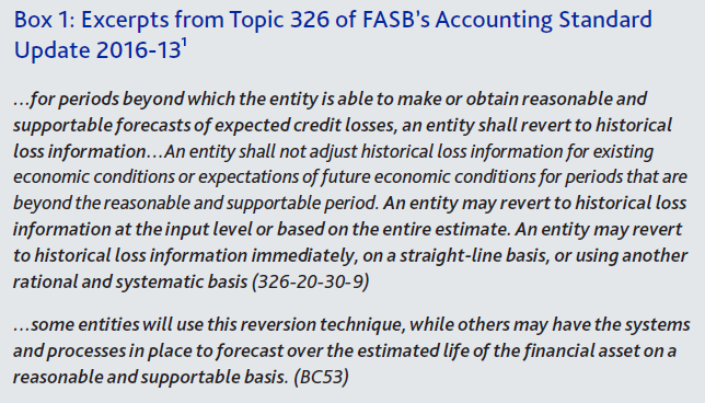
The Financial Accounting Standards Board guidelines require institutions to revert to their historical losses beyond the reasonable and supportable forecast horizon (see Box 1 above), but do not prescribe a specific approach or methodology. This lack of specificity is understandably causing angst among institutions trying to build a CECL-compliant accounting process in time for the 2020 adoption deadline for Securities and Exchange Commission-registered institutions. With the CECL guidelines on mean reversion open to multiple interpretations, our paper discusses some approaches institutions can take for reversion beyond the reasonable and supportable horizon. Our paper also describes the mechanism through which mean reversion occurs in the forecasts produced by the Moody’s Analytics Global Macroeconomic Model.
FASB guidelines on mean reversion
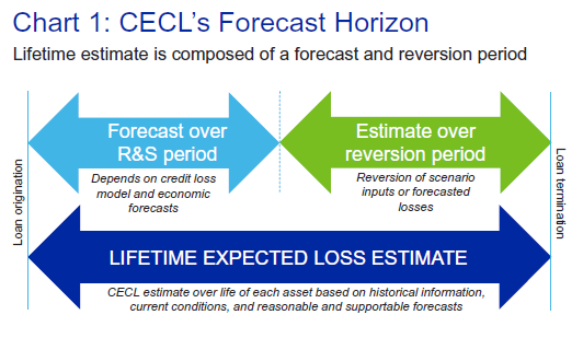
CECL requires a lifetime estimate of losses calculated from the time of origination and updated in each reported quarter for the losses expected over the remaining life of each loan, conditional on historical information, current conditions, and reasonable and supportable forecasts. The guidelines accommodate the concerns of institutions that they will be unable to produce reasonable forecasts over the full lifetime of the loans on their books. Rather than allowing institutions to limit their loss estimates to their own determined forecast horizon, FASB elected to maintain the definition of a full lifetime estimate composed of both a forecast and a reversion period (see Chart 1). Essentially, institutions are expected to forecast their losses for as far out as they can using reasonable and supportable forecasts and be able to defend their choice to auditors and regulators. After that time period, institutions should estimate future losses based on a reversion to historical information. The guidelines are nonprescriptive in terms of how the reversion is conducted, noting that institutions may opt to either revert the inputs into their forecasts or the outputs.
Input vs. output reversion
Interpreted simply, the guidelines allow for reversion at either the input, or economic forecast level, or at the output, or loss-rate level.
Under input reversion, economic forecasts revert to their historical trends after a certain number of forecast quarters. So, forecast credit loss rates based on these economic forecasts will converge to a constant unless other noneconomic dynamic variables, such as age, are included in the model.
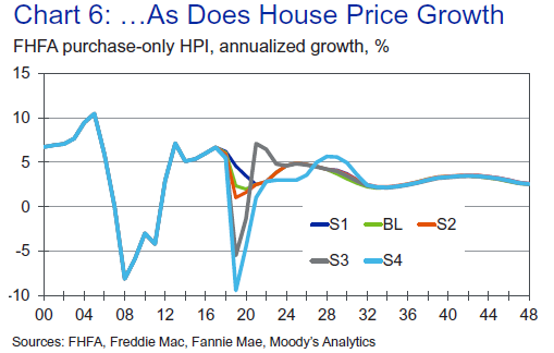
Macroeconomic forecasts usually begin to move toward their long-run equilibria after a reasonable forecast horizon, since most macroeconomic models do not attempt to predict turning points in the economy. The timing and speed of the reversion, however, depend on the variable in question and the forecast. For example, house prices typically take longer than interest rates to return to their equilibrium growth rates after a contraction, though specific recovery times are scenario-specific. The reversion process will usually take longer the further away the forecast is from the historical mean. For example, forecasts under stress scenarios will take longer to revert to their historical means compared with baseline forecasts, which are likely to be closer to the long-run equilibrium. How the Moody’s Analytics Global Macroeconomic Model handles reversion to historical means is discussed in detail later in the paper.
One argument against adopting input reversion is that it may under-predict credit losses far out into the future. Credit losses tend to be convex, nonlinear, and asymmetric. Simply put, losses under an optimistic scenario may not deteriorate significantly relative to a baseline scenario. Borrowers who were not driven to default when house prices were rising at 5% will continue not to default when house prices are rising at 15%. However, losses may rise exponentially when the economy contracts. The erosion in homeowner equity when prices are falling at 5% may lead to a sharp increase in the number of defaults. The counterpoint to this argument is that most losses stem from the short-term forecast. Far out into the future, many of the current loans would have either matured or reached the end of their life, where the probability of them defaulting would be extremely low.
We recommend input reversion as a mean reversion approach only if the economic forecast models and the credit loss models are deemed fit enough to produce reliable forecasts over the life of the loan, say 30 years. “Reliable” here means stable and reasonable, given the information we have today. It does not mean accurate predictions of future business cycles—that would be impossible to do based on today’s information. However, if economic and credit-loss models are not satisfactory, then input reversion is not recommended, and institutions should adopt output reversion instead.
Under output reversion, entities will revert to their historical losses beyond a certain reasonable period. That is, they will ignore the economic forecasts beyond a certain horizon and overlay the loss rates produced by their credit models with the historical loss rates. This overlay can happen instantaneously or gradually over a couple of quarters. Chart 2 shows an example comparing the loss rates under input and output reversion.

Reverting in outputs might seem like a shortcut, since it involves using the loss models for only a few years before overlaying with the historical loss rates. But in reality, the approach is quite complex and requires making and defending multiple assumptions, especially around portfolio segmentation and the historical look-back period. This becomes quite onerous if the institution has a new or changed portfolio with very little history or with adequate history but with few or no defaults. In such cases, it is hard to find a historical average to revert to that can be defended in front of auditors and regulators. In the absence of adequate history, the institution could certainly look at loss rates for peer groups—but then the choice of the peer group will also need to be explained.
Mean reversion in the Moody’s Analytics Global Macroeconomic Model
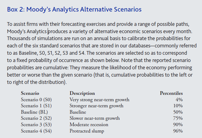
Moody’s Analytics maintains a Global Macroeconomic Model that forecasts more than 10,000 globally interlinked economic and financial time series that collectively account for 95% of global economic activity.2 The model is delivered through the Scenario Studio web-based platform that enables real-time interactive collaboration on economic scenarios or forecasts among multiple concurrent users. The model consists of a single, simultaneous system of structural economic equations that allow for a variety of cross-country interactions through demand, price, and financial market linkages. The model equations are all specified according to established macroeconomic theory, with parameters estimated econometrically using historical data. A baseline and a number of alternative scenario forecasts are produced at a quarterly frequency, extending over a 30-year time horizon. See Box 2 for a description of the Moody’s Analytics alternative scenarios. These forecasts are updated each month to retain consistency with the most recent economic data and are fully documented and transparent, supported by rigorous governance processes that stand up to regulatory and audit scrutiny. Advanced technology in the Scenario Studio platform helps clients generate scenarios required for regulatory compliance and accounting standards such as the Comprehensive Capital Analysis and Review, Internal Capital Adequacy and Assessment Process, IFRS 9, and CECL.
Financial institutions, governments, and corporate clients can use the Global Macroeconomic Model to determine the impact of domestic and foreign economic shocks. The model accounts for trade flows, financial market conditions, migration, commodity prices, and foreign investment. It captures the complexity of the global economy and demonstrates that the economic impacts of government policy changes and geopolitical events are much larger and reverberate more broadly across the globe and for longer than is commonly thought.
Reversion dynamics in the Moody’s Analytics Global Macroeconomics Model depend on the specific economic indicator under consideration. Some factors adjust quickly to economic shocks, while others tend to undergo a longer adjustment period. Each indicator is examined and modeled individually within the system of the global model in order to capture these specific dynamics. That being said, as a general rule the forecasts across the alternative economic scenarios tend to revert toward their long-term equilibrium trends within two to three years from the forecast start date.
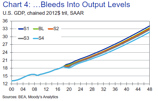
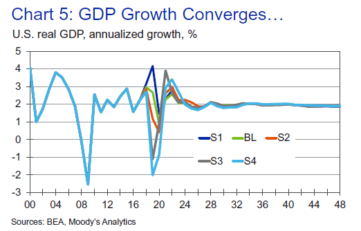
We illustrate the model’s reversion mechanism through three key economic indicators for CECL loss forecasting: the unemployment rate, real GDP, and house prices. We observe that in the alternative scenarios produced in September 2018, the unemployment rates reach their peak or trough within nine quarters from the start of the forecast. The unemployment rate bottoms out at 3% in Q42019 in the 10th percentile upside scenario, S1, and peaks at 8.3% in Q42020 in the 96th percentile downside scenario, S4, as shown in Chart 3. This range provides users of the forecast the ability to examine the impact of convexity on their credit loss forecasts.
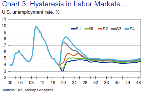
After reaching either their peak or trough, the unemployment rates in each of the scenarios converge to their long-run equilibrium over a period of two to eight years. The extended period of time is consistent with historical observation: It usually takes the labor market the better part of a decade to return to full employment after episodes of deep contraction. Notably, the speed of reversion depends on the state of the economy at the start of the forecast. If the economy is already near equilibrium, then the time to recover will be shorter than if the economy is either overheating or in recession.
The astute reader may observe that the unemployment rate across the scenarios does not converge to a single level or path. There is a small level shift, with the rate in S1 converging to 4.5% by 2048 and the rate in S4 converging to 4.9%. The difference is due to an inherent assumption of hysteresis, which posits that a period of high unemployment will permanently increase the equilibrium or natural rate of unemployment otherwise known as the non-accelerating inflation rate of unemployment.3 One cause of hysteresis may be the loss of skills by unemployed individuals, so that even when the economy improves, some workers remain permanently unemployed. Another theory posits that the bargaining power of workers employed during a recession strengthens because of their reduced numbers. As the economy improves, these workers bargain for higher wages, at the cost of increased employment. Yet another hypothesis is that the forces that drive long-term growth—investment in physical capital, research and development expenditures, and adoption of new technologies—slow down during recessions, causing permanent damage to the economy’s output-generating capacity. It should be noted that although hysteresis is assumed in the Moody’s Analytics forecasts, its impact is mild, resulting in a small difference in equilibrium levels across scenarios. To the extent users of the global macroeconomic forecasts do not wish to incorporate hysteresis in their views, the scenarios are easily overwritten.
Summary
FASB’s guidelines around reversion to historical losses beyond the reasonable and supportable forecast horizon are nonprescriptive and therefore open to interpretation. They allow for reversion in either economic inputs or loss outputs. Neither approach is ideal, and whichever is chosen will need to be defended as being the most suitable for the institution’s own portfolio, data, and models.
With respect to input reversion, and the spirit of CECL in general, the Moody’s Analytics Global Macroeconomic Model is consistent with the guidelines. The alternative scenarios produced by the model embody reasonable and supportable forecasts over a period of one to three years followed by a reversion to long-term trends afterward. The model does not attempt to forecast expansions or contractions beyond the next business cycle, which would be neither reasonable nor supportable. By incorporating multiple scenarios into their loss estimation process, users of the Moody’s Analytics scenarios can address the issue of forecast uncertainty that the CECL standard is attempting to capture.
1 https://asc.fasb.org/imageRoot/39/84156639.pdf
2 See “Moody’s Analytics Global Macroeconomic Model Methodology” by Mark Hopkins, Moody’s Analytics Regional Financial Review (June 2018) for a description of our global macro model.
3 See https://voxeu.org/article/hysteresis-and-fiscal-policy-during-global-crisis for a review of the literature on hysteresis.


